Introducing Tidyverse-Part 2: %>%, the Forward Chaining
By Ou Zhang in R Data science
May 22, 2020
Figure 1: Pipe Operator
Hi, I'm the here-bot cat!
Use me to find your way in your website.
- Here I am:
- content/blog/2020-05-22-pipe-forward-chaining/index.html
- Here is my R Markdown source file:
- blog/2020-05-22-pipe-forward-chaining/index.Rmd
You'll want to edit this file, then re-knit to see the changes take effect in your site preview.
To remove me, delete this line inside that file: {{< here >}}
- My content section is:
- blog
- My layout is:
- single-sidebar
- Images in this page bundle:
- /blog/2020-05-22-pipe-forward-chaining/featured.jpg
- /blog/2020-05-22-pipe-forward-chaining/img/intermediate.PNG
- /blog/2020-05-22-pipe-forward-chaining/img/pipe.PNG
- /blog/2020-05-22-pipe-forward-chaining/img/pipe_example.png
Instead of introducing tidyr and dplyr packages-two most essential R packages for data wrangling, I would like to insert a side topic that I think it’s worth to mention for R programming efficiency as my 2nd Tidyverse blog 1. To me, this important programming command completely changes my view of programming and reshapes my programming habit since I used it. This magic command is %>%, a.k.a: the pipe operator.
The hot key for
%>%in RStudio isCtrl+Shift+M.
%>% comes from the magrittr package that allows you to express a sequence of multiple operations. The magrittr package was created by Stefan Milton Bache and, in Stefan’s words, has two primary aims: “to decrease development time and to improve readability and maintainability of code.” It can greatly simplify your code and make your operations more intuitive.
Backward Chaining - the traditional program way
Before %>% was invented, most of the programming logic flows including R program is like this:
results <- operation(object)
Basically, the result is the output assigning from the right side after operation command operating the object. The object, most often, is the dataset.
The logic flow is from right to left and is called backward chaining. Because of this backward chaining feature, there are multiple ways for the traditional programming.
Let us refresh how we create a statistical program in a traditional way.
Traditional programming way 1: Intermediate steps
The first and simplest way is to save each step as a new object:
     a <- filter(data, variable == numeric_value)
     b <- summarise(a, Total = sum(variable))
     c <- arrange(b, desc(Total))
So, in order to obtain the final output - c, the intermediate output - a and b are created step by step. The main downside of this approach is that it forces you to name each intermediate element. That leads to two problems:
The code is cluttered with unimportant names
You have to carefully increment the suffix on each line (i.e., temp1, temp2, temp3, etc.)
Whenever I write code like this, I invariably use the wrong number on one line and then spend hours scratching my head and trying to figure out what went wrong with my code if the code structure is complex. Sometimes, I even need to write down all the intermediate output names on paper so that I can keep tracking the program logic flow.
Traditional programming way 2: Overwrite the original
The second way is to overwrite the original object at each step:
     a <- filter(data, variable == numeric_value)
     a <- summarise(a, Total = sum(variable))
     a <- arrange(b, desc(Total))
This is less typing (and less thinking), so you’re less likely to make mistakes. In the example, after each step, the old result - a is replaced by the new result - a. It sounds straightforward right? However, there are two major problems:
Debugging is painful: if you make a mistake you’ll need to re-run the complete pipeline from the beginning.
The repetition of the object being transformed (I’ve written a three times!) obscures what’s changing on each line. And what’s worse, you really can’t tell what the
aobject looks like inside without clicking-in the object.
Traditional programming way 3: Function composition or Nested Structure
The third way is to abandon assignment and just string the function calls together. This is also called nested option. This apprach strings all the function calls together into a single object and ignore assigning it anywhere.
    # Example 1:
    arrange(
            summarize(
                filter(data, variable == numeric_value),
                Total = sum(variable)
            ),
        desc(Total)
    )


   # Example 2:
    arrange(summarize(filter(data, variable == numeric_value),Total = sum(variable)),desc(Total))
I have seen a lot of experienced programmers doing this with or without changing lines. They may think this is efficient, since it includes all the functions they need to do analysis, but also keep everything in one line or so.
However, this nested option pattern gives me the most headache. Programmers like me (not very smart, not very good at processing speed), have the hardest time to deal with this nested option. The biggest disadvantage is that you have to
- read from inside-out,
- from right-to-left, and that
- the arguments end up spread far apart (evocatively called the
dagwood sandwhich problem).
In short, this code is hard for a human to consume.
Forward Chaining - the %>% way
Basic %>% process
In general, %>% take the output from one function and feed it to the first argument of the next function. Let’s see how %>% operates the commands in the example.
# pipe way
data %>%
  filter(variable == "value") %>%
  summarise(Total = sum(variable)) %>%
  arrange(desc(Total))
If you’ve never seen %>% before, you’ll have no idea what this code does. But the logic is so intuitive and straightforward.
You can read this as you would read normal prose (we read the %>% as “and then”):
"
take dataand thenfilterand thensummarize**and then*arrange."
%>% forward a value, or the result of an expression, into the next function call/expression. This is also called forward chaining.
object %>% operation() -> resultThis process is so efficient in that it doesn’t save unncessary objects (as in intermediate option) and performs as effectively (as both overwrite option and nested option) but makes your code more readable in the process.
Here is another example to explain the ‘pipe’ to newbies…
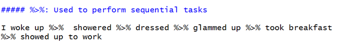
Figure 2: simple pipe example
Extract intermediate output in %>% process for QC
So, you’ve watched basic %>% process from the last section. Are you convinced to use pipe? It sounds promising, right? But data scientists, like me, always want to check the intermediate results to ensure calculation at each step is accurate and in line with what I expect. How could we do this intermediate result check in the %>% process?
Here is what you could do. You first include the initial data and all intermediate steps you want to run, then click run, the result saved in the R console is the intermediate result you would like to investigate (see the example below).
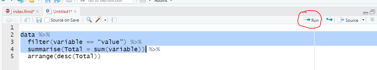
Figure 3: Check intermediate result
Functions in %>% chain not the first argument
When using the %>% operator the default is the argument that you are forwarding will go in as the first argument of the function that follows the %>%. However, in some functions the argument you are forwarding does not go into the default first position. In these cases, you place “.” to signal which argument you want the forwarded expression to go to.
data %>%
        filter(carb > 1) %>%
        lm(mpg ~ cyl + hp, data = .) %>%
        summary()
When to use the %>%
Now, you’ve read a lot of good things about %>%. You may ask when should I use this operator. Here are some suggestions from Bob Rudis speech-“Writing Readable Code with Pipes” at rstudio::conf 2017.
- the chain should be
> 1 - a pipe group should be designed to accomplish a unified task
- it’s OK to change object class/type/mode
- be data-source aware
- Pipe operations should be “atomic”
- pipe (briefly) in pipe
- Don’t be reticent to create new verbs
- keep them short
In addition, Bob Rudis’s speech also connects super Mario with pipe. If you are interested, you can find his talk from the link below. I highly recommend you to watch this talk. It’s so fun!
Writing Readable Code with Pipes (Bob Rudis,rstudio::conf 2017)
When not to use the %>%
So, the %>% is a powerful tool, but it’s not the universal tool, and it doesn’t solve every problem! Here are some situations that you should reach for another tool:
Your pipes are longer than (say)
10steps. In that case, create intermediate objects with meaningful names. That will make debugging easier, because you can more easily check the intermediate results, and it makes it easier to understand your code, because the variable names can help communicate intent.You have
multiple inputs or outputs. If there isn’t one primary object being transformed, but two or more objects being combined together, don’t use the pipe.You are starting to think about a directed graph with a complex dependency structure.
%>%are fundamentally linear and expressing complex relationships with them will typically yield confusing code.
Additional Pipe Operators
magrittr also offers some alternative pipe operators, Such as:
%<>%: result assigned to left hand side object instead of returning it%$%: expose names within left hand side objects to right hand side expressions%T>%: allows you to continue piping functions that normally cause termination
Since they are not as popular as %>%, I will discuss them in a separate blog.
Conclusion
Finally, I got convinced that the pipe operator is one (if not THE) most important innovation introduced to the R ecosystem. I will use it as much as possible.
How about you?
The basic
%>%pipe is automatically imported as part of thetidyverselibrary. If you wish to use any of the extra tools frommagrittras demonstrated in R for Data Science, you need to explicitly loadmagrittr.↩︎